The code and model available on Github

With the imagery downloaded, the next step was to autonomously investigate these images for HV towers. We generated a probability score on the interval [0, 1] that a HV tower was present in each raster image using a convolutional neural network (CNN). The CNN took raster images as input, and produced a single probability per image as output. Specifically, we used the XCeption neural network (Chollet, 2016), as it has shown excellent scores on the ImageNet benchmark test set and has relatively few parameters relative to comparable CNNs (e.g., VGG and Inception). The latter fact implies faster training and prediction run-times simply because there are fewer point computations per image.

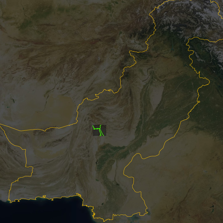
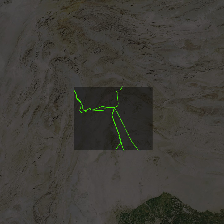
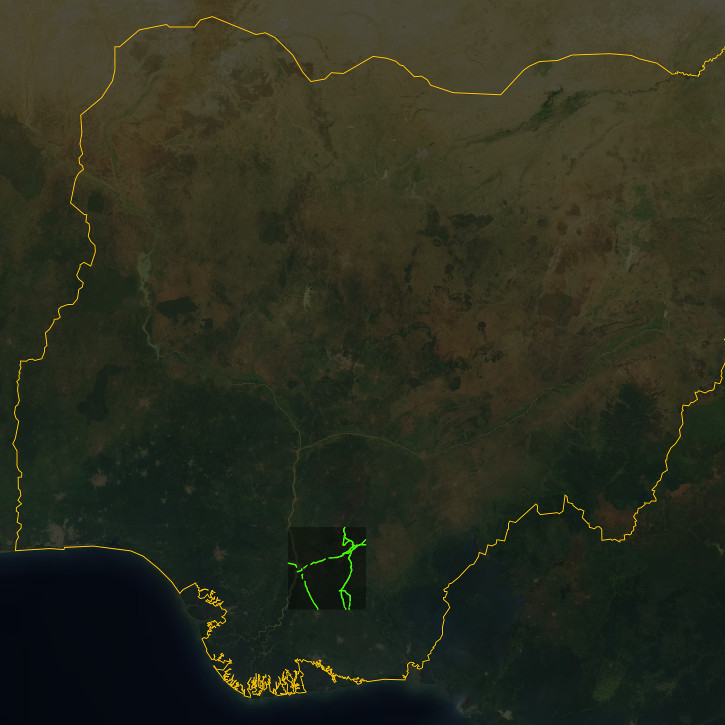
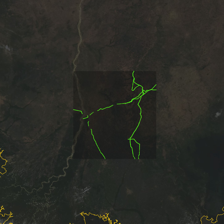
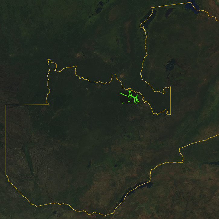
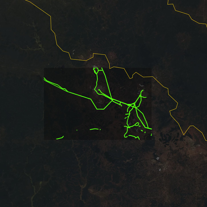
The XCeption model was trained using three small datasets -- one from each of the three target countries (Figures 5-7). The Data Team manually validated all tiles in these datasets and incorporated any required changes into OSM. This involved checking every meter of ground so that we were confident our training dataset did not miss any towers or include false positives, which would hurt our ML model performance during the inference stage (i.e., predicting on a country-wide image set). For the training data, we only used the Digital Globe Vivid layer as this was the imagery we had access to for full country prediction. We then constructed the actual data using Label-Maker -- an open tool we built previously to rapidly construct ML-ready datasets from OSM and an imagery source. The training procedure leveraged transfer learning: the XCeption model was initialized in Keras using weights from ImageNet training. We then re-trained only the top layer for 2-5 epochs so that it would output the probability of two classes (HV tower present or absent), and finally opened up training to all layers to fine tune the entire model.

In training, we used the binary cross-entropy loss function and generally trained over 15-30 epochs of the total training dataset. We also made use of Keras’s utility functions including early stopping and automatically reduced learning rate when validation loss hit a plateau. The dataset was augmented by using Keras’s image preprocessing functions to randomly flip, rotate, and scale original images during the training procedure. Results were visualized with Tensorboard to monitor model progress. For hyperparameters, we used the Hyperopt library to intelligently iterate over different hyperparameter combinations. The full list of hyperparameters is available in config.py, but generally this included options like the optimizer, learning rate, initialization strategy, etc. We selected an optimal model based on the highest accuracy score achieved on the held-out testing data across all Hyperopt iterations.

We carried out all country-wide predictions in the inference stage on AWS EC2 instances optimized for GPU compute. Specifically, we used the p2.xlarge and p2.8xlarge instance types and ran these as Spot Instances (as opposed to On-Demand) to reduce AWS costs. We typically ran 2-3 instances at a time to increase throughput. On each instance, we processed large batches of images one at a time. Each country was generally divided up into about 7-10 batches (according to the X-indices of tiles) as it was not feasible to transfer an entire country’s worth of tiles from S3 to the EC2 instance. While computing probability scores, the prediction script periodically uploaded tile prediction scores (as a JSON file) to S3 while processing (around every 5,000 images). This ensured that the prediction was fault tolerant -- scores were not lost when the instance shut down unexpectedly.