
Introduction to machine learning, neural networks and deep learning
Objectives
Understand the fundamental goals of machine learning and a bit of the field’s history
Gain familiarity with the mechanics of a neural network, convolutional neural networks, and the U-Net architecture in particular
Discuss considerations for choosing a deep learning architecture for a particular problem
What is Machine Learning?
Machine learning (ML) is a subset of artificial intelligence (AI), which in broad terms, is defined as the ability of a machine to simulate intelligent human behavior.
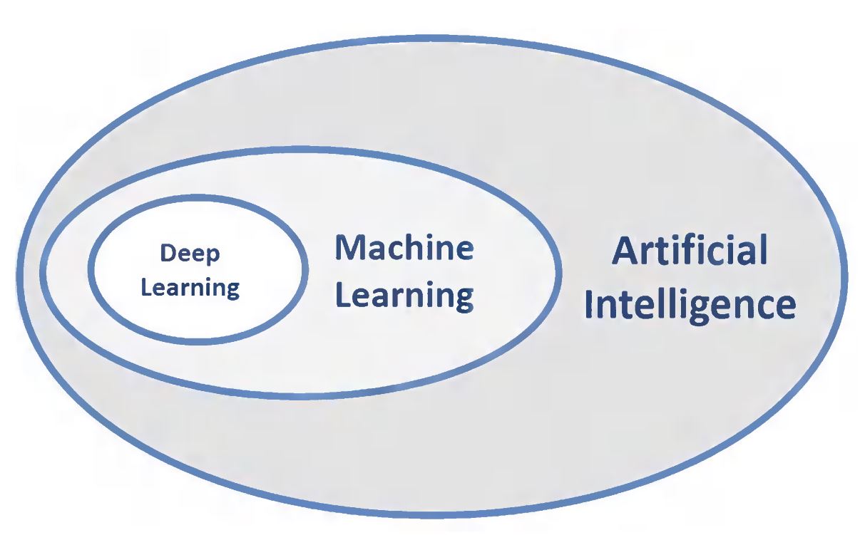
Fig. 1 AI, ML, DL.
Compared to traditional programming, ML offers:
time savings on behalf of the human programmer,
time savings on behalf of a human manual interpreter,
reduction of human error,
scalable decision making
ML requires good quality data, and a lot of it, to recognize key patterns and features.
Humans still have a role in this process, by way of supplying the model with data and choosing algorithms and parameters.
There are several subcategories of machine learning:
Supervised machine learning involves training a model with labeled data sets that explicitly give examples of predictive features and their target attribute(s).
Unsupervised machine learning involves tasking a model to search for patterns in data without the guidance of labels.
Important
There are also some problems where machine learning is uniquely equipped to learn insights and make decisions when a human might not, such as drawing relationships from combined spectral indices in a complex terrain.
What are Neural Networks?
Artificial neural networks (ANNs) are a specific, biologically-inspired class of machine learning algorithms. They are modeled after the structure and function of the human brain.
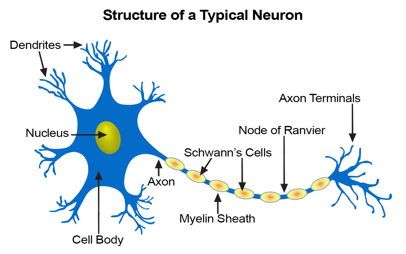
Fig. 2 Biological neuron (from https://training.seer.cancer.gov/anatomy/nervous/tissue.html).
ANNs are essentially programs that make decisions by weighing the evidence and responding to feedback. By varying the input data, types of parameters and their values, we can get different models of decision-making.

Fig. 3 Basic neural network from https://towardsdatascience.com/machine-learning-for-beginners-an-introduction-to-neural-networks-d49f22d238f9.
In network architectures, neurons are grouped in layers, with synapses traversing the interstitial space between neurons in one layer and the next.
What are Convolutional Neural Networks?
A Convolutional Neural Network (ConvNet/CNN) is a form of deep learning inspired by the organization of the human visual cortex, in which individual neurons respond to stimuli within a constrained region of the visual field known as the receptive field. Several receptive fields overlap to account for the entire visual area.
In artificial CNNs, an input matrix such as an image is given importance per various aspects and objects in the image through a moving, convoling receptive field. Very little pre-processing is required for CNNs relative to other classification methods as the need for upfront feature-engineering is removed. Rather, CNNs learn the correct filters and consequent features on their own, provided enough training time and examples.

Fig. 4 Convolution of a kernal over an input matrix from https://towardsdatascience.com/intuitively-understanding-convolutions-for-deep-learning-1f6f42faee1.
What is a kernel/filter?
A kernel is matrix smaller than the input. It acts as a receptive field that moves over the input matrix from left to right and top to bottom and filters for features in the image.
What is stride?
Stride refers to the number of pixels that the kernel shifts at each step in its navigation of the input matrix.
What is a convolution operation?
The convolution operation is the combination of two functions to produce a third function as a result. In effect, it is a merging of two sets of information, the kernel and the input matrix.

Fig. 5 Convolution of a kernal over an input matrix from https://theano-pymc.readthedocs.io/en/latest/tutorial/conv_arithmetic.html.
Convolution operation using 3D filter
An input image is often represented as a 3D matrix with a dimension for width (pixels), height (pixels), and depth (channels). In the case of an optical image with red, green and blue channels, the kernel/filter matrix is shaped with the same channel depth as the input and the weighted sum of dot products is computed across all 3 dimensions.
What is padding?
After a convolution operation, the feature map is by default smaller than the original input matrix.

To maintain the same spatial dimensions between input matrix and output feature map, we may pad the input matrix with a border of zeroes or ones. There are two types of padding:
Same padding: a border of zeroes or ones is added to match the input/output dimensions
Valid padding: no border is added and the output dimensions are not matched to the input

What is Deep Learning?
Deep learning is defined by neural networks with depth, i.e. many layers and connections. The reason for why deep learning is so highly performant lies in the degree of abstraction made possible by feature extraction across so many layers in which each neuron, or processing unit, is interacting with input from neurons in previous layers and making decisions accordingly. The deepest layers of a network once trained can be capable inferring highly abstract concepts, such as what differentiates a school from a house in satellite imagery.
Cost of deep learning
Deep learning requires a lot of data to learn from and usually a significant amount of computing power, so it can be expensive depending on the scope of the problem.
Training and Testing Data
The dataset (e.g. all images and their labels) are split into training, validation and testing sets. A common ratio is 70:20:10 percent, train:validation:test. If randomly split, it is important to check that all class labels exist in all sets and are well represented.
Important
Why do we need validation and test data? Are they redundant? We need separate test data to evaluate the performance of the model because the validation data is used during training to measure error and therefore inform updates to the model parameters. Therefore, validation data is not unbiased to the model. A need for new, wholly unseen data to test with is required.
Forward and backward propagation, hyper-parameters, and learnable parameters
Neural networks train in cycles, where the input data passes through the network, a relationship between input data and target values is learned, a prediction is made, the prediction value is measured for error relative to its true value, and the errors are used to inform updates to parameters in the network, feeding into the next cycle of learning and prediction using the updated information. This happens through a two-step process called forward propagation and back propagation, in which the first part is used to gather knowledge and the second part is used to correct errors in the model’s knowledge.

Fig. 8 Forward and back propagation.
The activation function decides whether or not the output from one neuron is useful or not based on a threshold value, and therefore, whether it will be carried from one layer to the next.
Weights control the signal (or the strength of the connection) between two neurons in two consecutive layers.
Biases are values which help determine whether or not the activation output from a neuron is going to be passed forward through the network.
In a neural network, neurons in one layer are connected to neurons in the next layer. As information passes from one neuron to the next, the information is conditioned by the weight of the synapse and is subjected to a bias. The weights and biases determine if the information passes further beyond the current neuron.
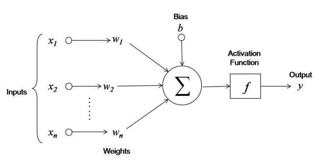
Fig. 9 Weights, bias, activation.
During training, the weights and biases are learned and updated using the training and validation dataset to fit the data and reduce error of prediction values relative to target values.
Important
Activation function: decides whether or not the output from one neuron is useful or not
Weights: control the signal between neurons in consecutive layers
Biases: a threshold value that determines the activation of each neuron
Weights and biases are the learnable parameters of a deep learning model
The learning rate controls how much we want the model to change in response to the estimated error after each training cycle

The batch size determines the portion of our training dataset that can be fed to the model during each cycle. Stated otherwise, batch size controls the number of training samples to work through before the model’s internal parameters are updated.
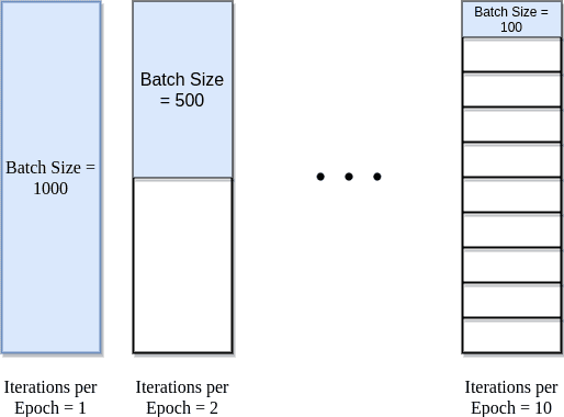
An epoch is defined as the point when all training samples, aka the entire dataset, has passed through the neural network once. The number of epochs controls how many times the entire dataset is cycled through and analyzed by the neural network. Related, but not necessarily as a parameter is an iteration, which is the pass of one batch through the network. If the batch size is smaller than the size of the whole dataset, then there are multiple iterations in one epoch.
The optimization function is really important. It’s what we use to change the attributes of your neural network such as weights and biases in order to reduce the losses. The goal of an optimization function is to minimize the error produced by the model.
The loss function, also known as the cost function, measures how much the model needs to improve based on the prediction errors relative to the true values during training.

Fig. 12 Loss curve.
The accuracy metric measures the performance of a model. For example, a pixel to pixel comparison for agreement on class.
Note: the activation function is also a hyper-parameter.
Common Deep Learning Algorithms for Computer Vision
Image classification: classifying whole images, e.g. image with clouds, image without clouds
Object detection: identifying locations of objects in an image and classifying them, e.g. identify bounding boxes of cars and planes in satellite imagery
Semantic segmentation: classifying individual pixels in an image, e.g. land cover classification
Instance segmentation: classifying individual pixels in an image in terms of both class and individual membership, e.g. detecting unique agricultural field polygons and classifying them
Generative Adversarial: a type of image generation where synthetic images are created from real ones, e.g. creating synthetic landscapes from real landscape images
Semantic Segmentation
To pair with the content of these tutorials, we will demonstrate semantic segmentation (supervised) to map land use categories and illegal gold mining activity.
Semantic = of or relating to meaning (class)
Segmentation = division (of image) into separate parts
U-Net Segmentation Architecture
Semantic segmentation is often distilled into the combination of an encoder and a decoder. An encoder generates logic or feedback from input data, and a decoder takes that feedback and translates it to output data in the same form as the input.
The U-Net model, which is one of many deep learning segmentation algorithms, has a great illustration of this structure.

Fig. 13 U-Net architecture (from Ronneberger et al., 2015).
In Fig. 13, the encoder is on the left side of the model. It consists of consecutive convolutional layers, each followed by ReLU and a max pooling operation to encode feature representations at multiple scales. The encoder can be represented by most feature extraction networks designed for classification.
The decoder, on the right side of the Fig. 13 diagram, is tasked to semantically project the discriminative features learned by the encoder onto the original pixel space to render a dense classification. The decoder consists of deconvolution and concatenation followed by regular convolution operations.
Following the decoder is the final classification layer, which computes the pixel-wise classification for each cell in the final feature map.
ReLU is an operation, an activation function to be specific, that induces non-linearity. This function intakes the feature map from a convolution operation and remaps it such that any positive value stays exactly the same, and any negative value becomes zero.

Fig. 14 ReLU activation function.

Fig. 15 ReLU applied to an input matrix.
Max pooling is used to summarize a feature map and only retain the important structural elements, foregoing the more granular detail that may not be significant to the modeling task. This helps to denoise the signal and helps with computational efficiency. It works similar to convolution in that a kernel with a stride is applied to the feature map and only the maximum value within each patch is reserved.
